How To Calculate Mean Particle Size From Sieve Analysis

Tabular array of Contents

• Description of Sieving Equipment & Operation
• How to Plot Grain Size Distribution Curve
• How to Plot Semi Log Graph for Sieve Analysis
• Sieve Assay Lab Study Discussion & Decision

The experiments described in this paper were undertaken primarily for the purpose of measuring the quality of work done in screening and sorting in American concentrating-mills for Prof. Richards' work on Ore-Dressing. For this purpose a series of samples of screened and sorted products was obtained from four different mills, and a plan was devised for sizing these products, and for tabular and graphic representation of the results. The results, together with discussions as to their significance, and then far every bit they serve to interpret the quality of manufactory-work, have already been published in the to a higher place-mentioned work, and it is not the purpose of this paper to indistinguishable the piece of work, except so far every bit is necessary to explicate and illustrate methods and appliances.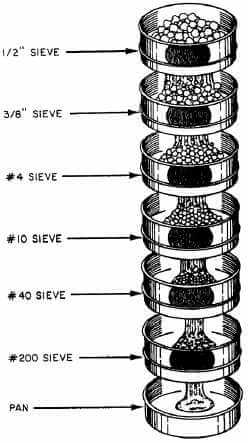

The sizing of coarse products was done by sifting on screens of sail-metal with circular punched holes. These holes ranged in size from 64 mm. to 0.5 mm. in diameter. Below the smaller limit, punched metal, suitable for this work, was not obtainable, and the sizing was carried on by sifting on woven wire-sieves. The finest woven wire-cloth obtainable gave a hole 0.073 mm. square, and the finest silk bolting-cloth gave a pentagonal pigsty with an average diameter of 0.069 mm. Even these very fine screens served no useful purpose in sifting certain of the very fine classifier-products, of which all, or nearly all, passed through the finest screen. A new adaptation of a method of settling and decantation with water in beakers was therefore worked out, and past this means the sizing was carried downward to grains of a diameter as small as 0.012 mm.

Description of Sieving Equipment & Operation

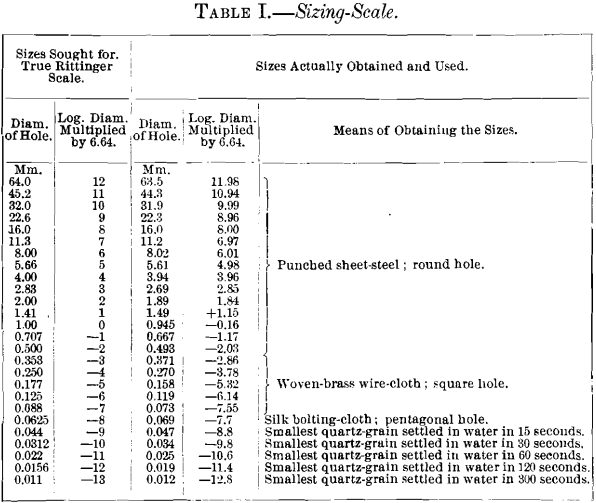
Sieves of sheet metal with circular punched holes were used equally far as practicable, chiefly considering, every bit already explained, the main object of the experiments was to test mill-work, and the mills had all used sheet-metal with round punched holes for coarse sizing and, farther, because the diameter of a circular pigsty is its only limiting dimension, whereas a foursquare hole may limit the passage of a grain of ore, according as the grain approaches, to take advantage of the diagonal dimension or the side dimension. The Rittinger sieve-scale was adopted as a standard for these sizing- tests, and screens were secured which would lucifer the sizes of the Rittinger calibration just as closely equally possible. The sizes of the Rittinger calibration are in geometrical progression. Diameters of successive sizes have a constant ratio of one.414, while the areas of holes of successive sizes have a constant ratio of 2.

The screens coarser than 2 mm. were measured with a scale, using a magnifying glass. Screens with holes 2 mm. in diameter and smaller, were measured nether a microscope, using a micrometer. From x to 20 holes were measured in each screen, and the average of these measures was taken to represent the size of hole for that screen. Sizes of square holes were determined by the mean of the measurements of the ii sides. Some of the holes in the woven wire, instead of being truly foursquare, were trapezoidal. In this example the long and short parallel sides were measured, and their mean length taken for one dimension. The sizing-scale used is shown in Tabular array I. The start cavalcade shows diameters in millimeters of the Rittinger sieve-scale, the third column shows the actual diameters of the holes in screens obtained for the piece of work in these experiments.

The samples were sifted dry, and the shaking and jarring on the sieves were carried on for such a time that the resulting weight of any size, expressed in per cent., should be meaning in the first identify of decimals. By trial information technology was found that on the punched screens, a iv-infinitesimal shaking was usually sufficient, while oft on the woven wire-screens two or iii times as long was needed; the time depending on the size of the sample and the area of the sieve. In sizing the finer products, it was found that samples weighing 200 grams for i sq. ft. of screening-surface could exist handled in a reasonable time, requiring somewhat less than ten minutes vigorous shaking and jarring.

In selecting a method of sizing for the material finer than 0.069 mm., we considered several methods. The employ of the analysis spitzlutte was not practicable, because of the very small water-currents necessary, the tediousness of the work, and the difficulty of separating the products, for weighing, from the relatively large bulk of water introduced. Certain experiments fabricated by Prof. W. O. Crosby in the sizing of samples of dirt were considered. He introduced a weighed portion of fabric in the superlative of a 0.5-in. glass tube, 5 ft. long, filled with water. The depth of the sediment was then measured at the stop of different periods upwards to one 60 minutes, and these depths were causeless

to stand for proportional weights. The sediment was then excavated from the tube to the points where measurements were taken, samples removed and the grains measured with a microscope-micrometer. This method was discarded chiefly considering the volumetric conclusion of quantities would be extraneous to mixtures of minerals of different specific gravity.

Allen Hazen has described a method of sizing applied to the examination of sand used in filtration-plants. A beaker was used in which 5 grams of the fine material was agitated with water, allowed to settle fifteen seconds and the water decanted. This was repeated past the addition of water iii times, yielding a settled product which was dried and weighed, and the boilerplate size of grain determined by measurement with a microscope-micrometer. The corporeality of overflow-product was non weighed, but was calculated by difference.

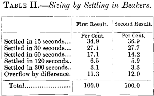
Following this idea, experiments were tried by settling successively for 300, 120, lx, thirty and 15 seconds. Samples of the five settled products were examined under the microscope to determine their uniformity and sizes. These results were so gratifying, and the sizes and then near those required for the Rittinger calibration, that the periods of settling named were adopted and a series of tests carefully conducted. A beaker 70 mm. in bore and 110 mm. deep was filled with distilled water to a depth of 90 mm., and 5 grams of ore, through a sieve with 0.069-mm. holes, was thoroughly stirred in. After standing quietly for 300 seconds, the water was quickly just carefully poured off without disturbing the settled material. The beaker was once more filled to the ninety-mm. marker and the procedure repeated. This was continued until the decanted water was clear. What remained in the beaker was similarly treated for periods of 120, 60, 30 and fifteen seconds in succession. Distilled water was used at a temperature of about 20° Cent. (68° Fahr.), and was not allowed to vary beyond 18° Cent, and 22° Cent. (64.4° Fahr. and 71.half dozen° Fahr.). Each product was allowed to settle, the clear water siphoned off, and the residues dried and weighed, except the finest product, which was determined by difference. Information technology was found, in lodge to make duplicate tests agree, that each period of settling (300, 120, threescore and 30 seconds) should be repeated the aforementioned number of times in the divide tests, and that information technology was non rubber to rely on the visual standard of the observer equally to the clearness of the terminal decanted h2o. Five settlings seem to give good results, and practice not take an unreasonable length of time; and while this plan was not adopted except during the latter part of the tests recorded in this paper, it is recommended as the well-nigh satisfactory method.

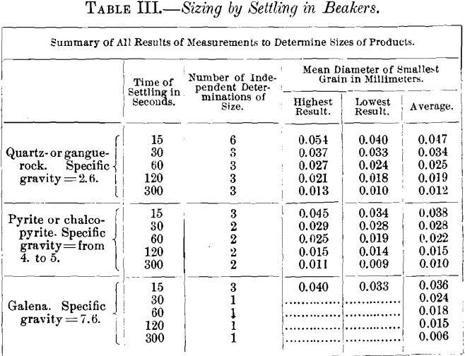
Table Ii. gives an idea of the degree of correspondence in results which are to be expected in sizing by settling in a beaker. Duplicate trials were made on the same sample, and the piece of work done on different days.

The sizes for the series of settled products were determined on the assumption that if the material were by and large quartz, practically the same quantities would have been obtained by screening and settling, if the screen-holes had the same diameters equally the smallest grains of quartz in each of the settled products. If the textile were mostly pyrite or mostly galena, the settled products would stand for in quantity to what would be obtained by dissimilar screen-sizes determined past measuring the smallest grains of pyrite or galena. If a sample under examination were made up of a mixture of quartz and a heavy mineral, in which neither greatly predominated, the product would exist sorted rather than sized, and information technology is possible to express merely an approximation to results which would have been obtained from sifting, past averaging the sizes of the minerals according to the judgment of the observer.

In sifting, information technology is axiomatic that the 2 bottom dimensions determine the ability of grains to pass a square or a round hole; whereas, when measuring the aforementioned grains under a microscope, they never present their shortest bore for measurement. This is illustrated by some measurements of the largest grains in the xv-second settled products. These grains had all been through a pentagonal hole with boilerplate bore of 0.069 mm., only ane sample showed the average diameter of the largest grains of quartz to be 0.100 mm., and of galena, 0.092 mm. The other sample showed the boilerplate diameter of the largest quartz-grains to be 0.105 mm., and of the chalcopyrite 0.096 mm. In the get-go of these determinations the average largest dimension presented was 0.120 mm., and the boilerplate smallest dimension was 0.080 mm.

The justification of the plan of measuring the smallest grains, in society to determine sizes, rests partly in the fact that their sizes requite results which harmonize with the information secured by sifting, and with them yield smooth curves in plotting. As no other plan seemed more practical, it was adopted.

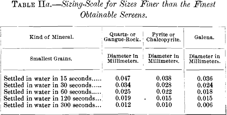
The diameter of the smallest particles in each settled production was determined equally follows: A sample was placed under a microscope with a micrometer-measuring attachment, and the length and width of the smallest particle in the field of the microscope was measured. This was washed with 20 or more separate fields for each sample, and the average of all measures was considered to correspond the smallest particle in the sample. Separate measurements were taken on quartz- or gangue-rock, pyrite or chalcopyrite, and galena. On quartz- products, samples were measured independently by two dissimilar observers, so as to eliminate the personal equation as far every bit possible. A summary of all these measurements appears in Table 3.

The quartz-sizes are used in the sizing-calibration, Tabular array I., and in the tabulated records of tests, because the major part of each sample consisted of quartz- or gangue-rock. The sizes for chalcopyrite or pyrite and galena are given in Table IIa. Chalcopyrite and pyrite are recorded together, because it was incommunicable to identify them in the samples and so every bit to measure them separately.

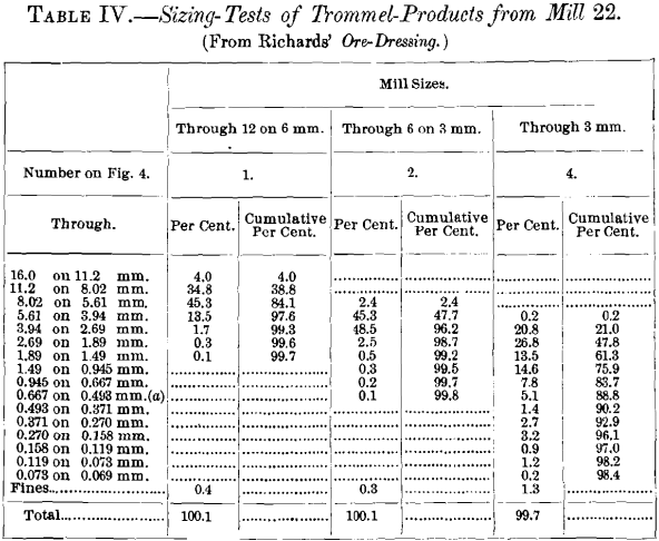
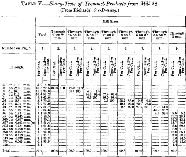
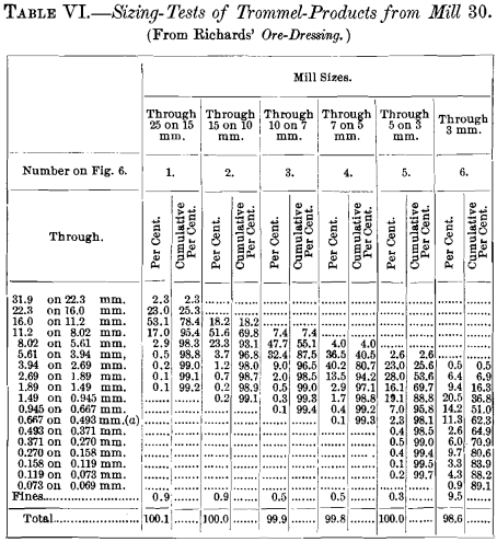
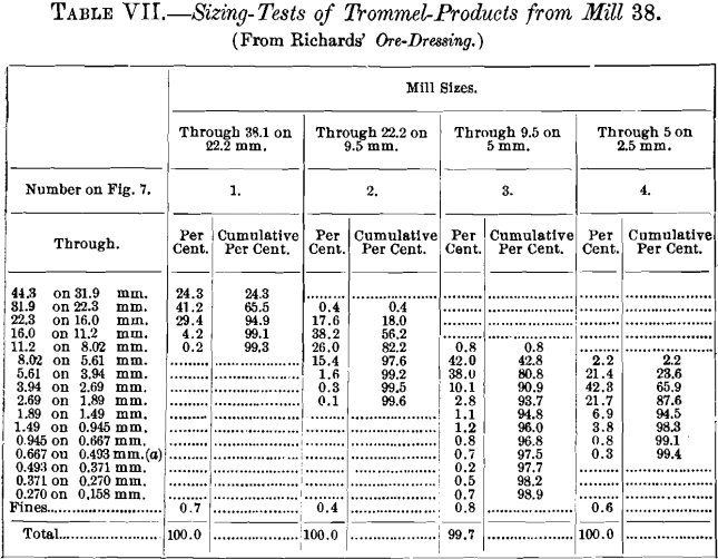
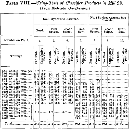
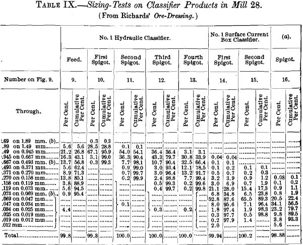
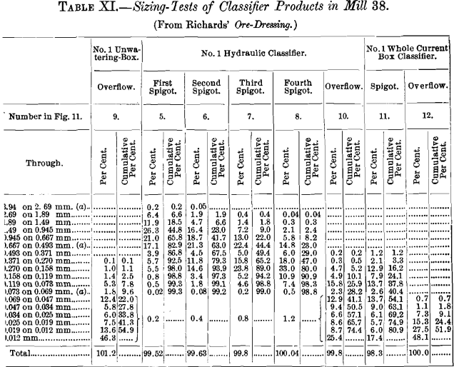
Complete tabulated results of the sizing of the mill products are shown in Tables IV. to Xi.

(a) Round-hole sieves were used downwards to and including 0.493-mm. size, and square holes for effectively sizes.

(a) Round-hole sieves were used downward to and including 0.493-mm. size, and square holes for effectively sizes.

(a) Round-hole sieves were used downward to and including 0.493-mm. size, and square holes for effectively sizes.

(a) Round-pigsty sieves were used down to and including 0.493-mm. size, and foursquare holes for finer sizes.

(a) Round-pigsty sieves were used down to and including 0.493 mm,; and so square holes down to and including 0.069 mm. Below 0.069 mm. settling in water was used, and the sizes given are diameters of quartz which settled a depth of xc mm. in 15, 30, 60, 120 and 300 seconds. All of the settled products independent some grains of mineral heavier than quartz, and these grains were smaller than the quartz-grains.

a) No. i whole current box classifier.

b) Round-hole sieves were used downwardly to and including 0.493 mm.; so square holes downward to and including 89 mm. Beneath 0.069 mm. settling in water was used, and the sizes given are diameters of quartz which tied a depth of xc mm. in fifteen, 30, 60, 120 and 300 seconds. All of the settled products contained some grains mineral heavier than quartz, and these grains were smaller than the quartz-grains.

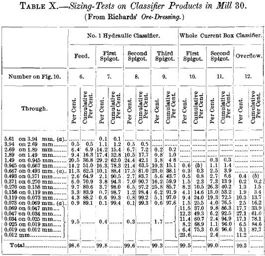
(a) Round-pigsty sieves were used downwardly to and including 0.493 mm.; then square holes downwardly to and including 0.069 mm. Below 0.069 mm. settling in h2o was used, and the sizes given are diameters of quartz which settled a depth of ninety mm. in 15, 30, 60, 120 and 300 seconds. All of the settled products independent some grains of mineral heavier than quartz, and these grains were smaller than the quartz-grains.

(b) This was all foreign fabric, such as chips, etc.

(a) Circular-hole sieves were used downwards to and including 0.493 mm.; and then foursquare holes downwards to and including .069 mm. Below 0.069 mm. settling in water was used, and the sizes given are diameters of quartz which settled a depth of ninety mm. in 15, thirty, 60, 120 and 300 seconds. All of the settled products contained some grains of mineral heavier than quartz, and these grains were smaller than the quartz-grains.

Sieve Assay Information Worksheet Download

How to Plot Grain Size Distribution Curve

In Tables Four. to 11. two columns of figures are given for each product. The numbers in the start column prove the pct, by weight of each size. The numbers in the second column, headed " Cumulative per cent.," show the total per cent, of the size and all coarser, and correspond the per centum of the whole sample which would rest on the screen, were it used lonely. The cumulative per cent, is particularly useful in the training of some of the graphic diagrams explained later.

A graphic method of representing sizing-tests, to be of value, should present the results in a class more readily interpreted and understood than the tabulated figures. The post-obit vi atmospheric condition are desirable in the graphic record:

1. The relative quantities betwixt the testing-screens should be clearly shown.
2. The relative quantities between screens of any ready of sizes other than that represented by the testing-screens should be apparent, and the actual quantities should be easy of decision by the utilise of a calibration.
3. The entire range of screen-sizes should be capable of representation in 1 effigy.
4. The predominating grain-size of the sample should be prominently apparent.
5. The form of the plot should exist unaffected by, and contained of, the sizing-scale used in making the test, thus affording, if desired, a ways of direct comparison with data secured past a dissimilar sizing-scale.
6. The method should exist uncomplicated, and the figures easily understood.

A number of methods take been used by other writers, and some of them will be discussed.

Prof. Courtney De Kalb, in his newspaper, Graphic Records of the Screening of Crushed Materials, presents a serial of drawings prepared by a method whereby the screen-sizes are plotted by measuring the diameters directly on a horizontal line, while the percentage of ore resting on each of the testing-screens is plotted vertically at the proper points.

Samples Nos. 1, 2, 3, 5 and 12 from Tables Vii. and XI. are adapted to a discussion of the various methods of graphic representation, and Fig. 1 shows a set of five curves prepared past this method, yielding what may be chosen an ordinary direct plot. These curves fulfill none of the requirements for graphic records except the showtime and last; and these they fulfill no amend than the tabulated figures. The omission of one of the sieves

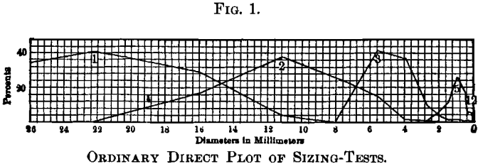
in making a test volition greatly change the form of the curve, which is considerably dependent on the sizing-scale used. While the method is all right for some kinds of data, information technology is not suited to represent sizing-tests, and is positively misleading in some particulars: For instance, curve No. 1 might be supposed to bespeak that if a xx-mm. screen had followed the 22.3-mm. screen, it would have retained 37 per cent, of the ore; but that

is cool, for the 16-mm. screen retained only 29.four per cent., and the xx-mm. screen would, of grade, neglect to retain sure sizes that were caught by the sixteen-mm. screen. Other forms of plot show that a 20-mm. screen would have retained 12.5 per cent, of the ore, a fact which this curve affords no means of determination.

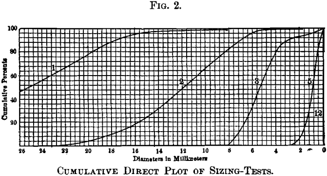
Luther Wagoner, in a paper, The Theory of Ore-Crushing, uses a method wherein the scale of sizes is laid off on a horizontal line just equally in the offset described method, but the quantities are represented past indicating cumulative percentages on the vertical calibration. The curves in Fig. 2 are fatigued past this method, and this form of plot may be chosen a cumulative direct plot. Its use is illustrated by reference to curve No. 2, from which may be read that 18 per cent, of the cloth under exam is coarser than xvi-mm., 50 per cent, coarser than 12-mm., and 82 per cent, coarser than 8-mm. size.

This method of graphic representation answers most of the requirements, simply information technology possesses i serious fault, in that information technology does non permit the representation of the entire range of sizes in i diagram. This is illustrated by Fig. 2, in which, at the scale adopted, bend No. two shows to practiced advantage, but this scale is likewise large to let curve No. 1 to appear on the sheet without extending it as far over again to the left, and at the aforementioned time, the scale is and so modest that curve No. 12 appears only as a vertical line. The cumulative straight plot recommends itself for its simplicity, and it will serve excellently for the written report of data secured from the sizing of single samples in which the range of sizes does not exceed a ratio of four to 1 betwixt diameters of coarsest and finest grains. Beyond these limits the curves are distorted to such an extent that the method is of little use.

The ratio of the openings in successive sizes of screens, as near as tin exist adamant, is almost 1 to one.41 for both fine and coarse screens; but, of course, the actual difference of the area of openings represented by this ratio is greater for the coarse than for the fine screens.

How to Plot Semi Log Graph for Sieve Analysis

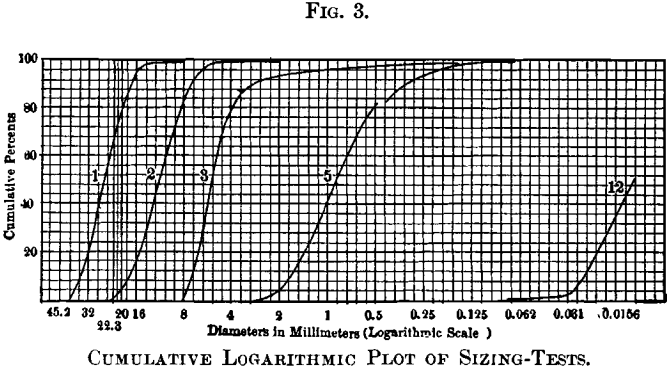
Information technology is desirable to have a method of plotting, in which equal distances on the plot correspond equal, ratios of diameter, or, if nosotros had been able to match the Rittinger scale precisely in getting the diverse sizing-screens, the data would be plotted at equal intervals on the horizontal calibration, thus compressing the curve at the large stop, and stretching the distances out on the small stop. The same result is secured automatically by plotting the logarithms of the diameters on the horizontal line, and Fig. 3 represents this method applied to the same information already presented by the other methods. If the logarithms of the diameters are multiplied by the abiding 6.64, numbers very convenient for plotting are secured, because they are whole numbers for the diameters of the Rittinger scale, and these multiples of the common logarithms are given in Table I. for convenience in plotting. The negative quality of the logarithm of all numbers less than unity must exist kept in mind, and since the logarithm of unity is zero, the original indicate for the scale of sizes volition be at the unit diameter, and smaller sizes volition exist scaled to the right and larger sizes to the left from that point. This form of plot may be called the cumulative logarithmic plot. It has been used past the Massachusetts Land

Board of Health for plotting sizing-curves of filtering-materials.

The curves resulting from this method fulfill every requirement for graphic representation. Its compliance with the starting time two requirements is easily shown by reference to curve No. ane in Fig. 3. Nosotros read that 78 per cent, of the sample is coarser than a 20-mm. screen, and that 65.5 per cent, is coarser than a 22.iii-mm. screen, therefore 12.5 per cent, of the material will fall between these sizes. It is also axiomatic that the steep portions of the curve show the range of predominant sizes. Referring again to curve No. 1, we see that 95 per cent, of the sample falls betwixt 16 mm. and 40 mm., and by curve No. 5, it appears that 75 per cent, of the sample is quite uniformly distributed between 0.5 mm. and ii mm.; too, that while some of the sample is probably as coarse as 2.8 mm.; as well, 4 per cent, is coarser than 2 mm., and although some grains are as fine as 0.062 mm., simply 20 per cent, is finer than 0.five mm., and but 6 per cent, effectively than 0.25 mm.

This method of graphic representation besides affords a ways of translating the records into tabular form to any scale of sizes which may be desired. The screens used in these tests conform only approximately to the Rittinger scale, but if information technology is desired, these results may be translated so that the tabular tape volition prove the results which would take been obtained if screens conforming precisely to the Rittinger calibration had been used. Such a translation of Table VII. has been made and is shown in Table XII.

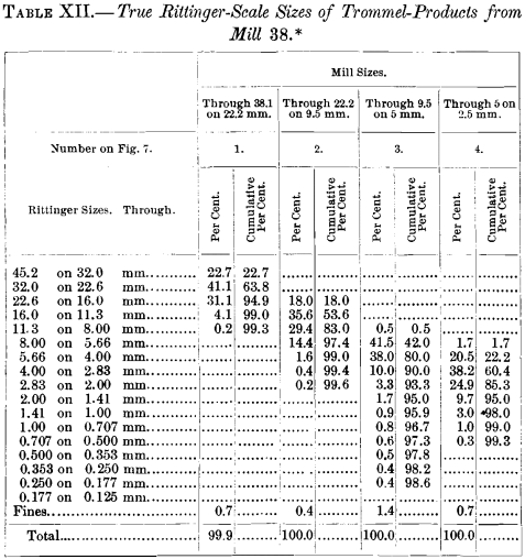
Tabular records are probably easier of comprehension to well-nigh readers than are the graphic diagrams, and it may be desirable to translate all sizing-records to one standard, thereby making possible, directly and easily understandable comparisons. Such a translation of whatsoever sizing-record is possible, provided the dimensions of the holes in the testing-screens are known.

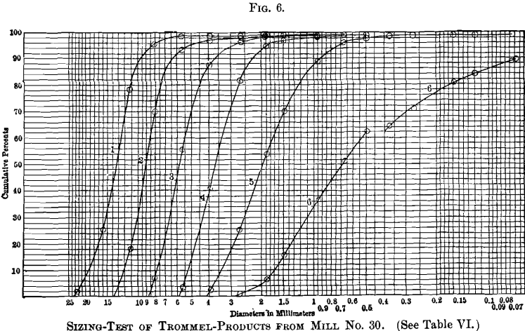
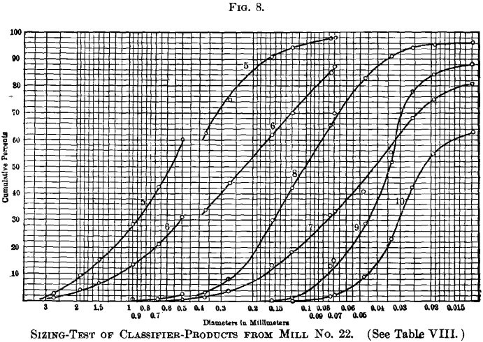
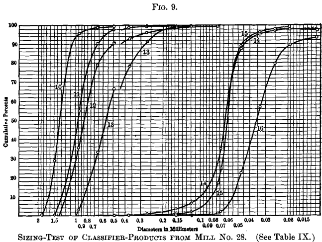
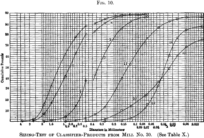
The cumulative logarithmic method of graphic representation was used by Prof. Richards to stand for all the tests recorded in this paper, and the plotted curves are reproduced in Figs. 4 to 11, inclusive. These curves-differ from those in Fig. 3, used

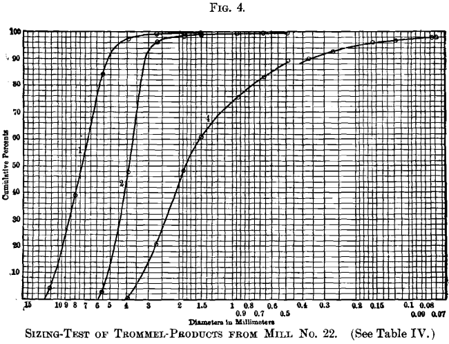
for illustrating the method, in that they are plotted on logarithmic paper ruled for the purpose. Diameters in millimeters may be read straight from the horizontal scale. The original drawings showed the position of each size of the Rittinger scale by vertical colored lines, but they could not exist reproduced in these engravings without confusion.

Information technology will exist noticed on Figs. four to 11, that for every sample containing material between 0.493- and 0.371-mm. size, at that place is a break in the curve at that point. In explanation of this, attention is directed to the fact already stated, that the 0.493-mm.

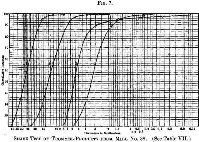
and all coarser screens have round holes, while the 0.371-mm. and all effectively screens have square holes. A round-pigsty screen will retain effectively textile and, therefore, more textile, than a square-hole screen of the aforementioned nominal size; consequently, if the fine screens could take been obtained with circular holes, or if the square-hole screens had been used throughout, the curves would be continuous and unbroken, without suffering whatsoever alteration of form or management. It is, therefore, believed to be amend to sacrifice whatever advantage pertains to the use of circular-hole screens, for those cases in which sizes smaller

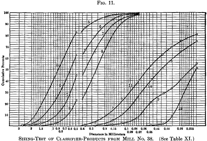
than 0.5 mm. enter into the problem; and it is then recommended to use foursquare-hole screens for all sizes.

The altitude which either part of the curve must exist moved, parallel to the scale of sizes, to bring the 2 curves together, will correspond the practical difference in constructive size, regarding screening-qualities, between round and square holes of the same nominal size. Past this means, the diagrams indicate that a foursquare pigsty, to retain but the aforementioned proportion of the sample equally a round hole 0.500 mm. bore, will measure from 0.406 to 0.435 mm., the first dimension beingness deduced for Mills Nos. 22 and 30, and the latter dimension for Manufactory No. 28.

This difference is probably due to some persistent difference in the shape of the grains of the mineral. Flat grains retained past a circular hole will be readily passed past the diagonal dimension of a square pigsty of the same nominal size; and a departure in the proportion of flat and splinter-shaped grains will explicate the deviation noted. Such a difference in the shape of grains in unlike mills is not surprising, and might be due to the cleavage of the ore, or, perchance, in part, to some difference in the methods of burdensome.

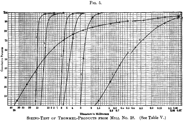
It will be noticed that no curves announced on Fig. five respective to Nos. ane and 2 on Table Five. These tests were on samples of very closely sized trommel-products, and the data replenish merely one plotted point for No. 1, and just two points for No. ii, neither beingness sufficient to yield a curve. A more than closely spaced sizing-scale, or intermediate screen-sizes, should have been used for these, also for tests Nos. five, 6, and 8, Table 5. and Fig. v, in each of which more than than 50 per cent, appears in the outset size, yielding, therefore, no plotted point most the line of naught per cent.

Another method of graphic representation was considered and discussed in connexion with these experiments; and while its nature does not recommend information technology for such general utilise as the cumulative direct plot, it has, nevertheless, some interesting and useful qualities.

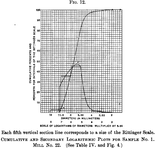
Referring to Figs. 12 and 13, the rising curves are identical with curves No. one, Fig. iv, and No. 5, Fig. 8, for Mill No. 22, except that the diameters are plotted by the same method as in Fig. 3, but on a larger scale. The heavy vertical section-lines represent to the sizes of the Rittinger scale.

The steps in the curve are fabricated by plotting on the vertical scale the percentages which would have rested on each sieve of a precise Rittinger scale. These figures are deduced by the method explained for Table XII.; and the height of each pace, measured by the vertical scale on the left, represents the percentage, if sized by the true Rittinger scale. On the scale of logarithms, the horizontal length of each step is unity, and the area of the rectangle between ii adjoining Rittinger sizes, divisional past the step and the base of operations line, is equal to the percentage of that size. These rectangles represent in a pictorial style the relative distribution of sizes in the samples, where the ratio betwixt successive sizes is compatible.

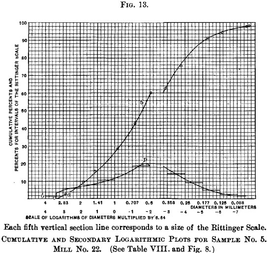
A comparison of this stepped effigy, with the master curves from which it is derived, shows a certain inconsistency at the starting-bespeak on the left, where the chief curve leaves the base-line at an abrupt angle. If these two figures are to be consistent, either the primary curve should curl up at the lower finish and extend to the point b, or the stride at that point should not extend to the left beyond the betoken where the principal curve touches the base line at c. The data furnish no means of determining just how the primary curve should keep from the nearest plotted point a to the base line. We have, still, on bend No. 4, Fig. 4; bend No. 7, Fig. five; curves Nos. 2 and three, Fig. 7; and curves Nos. 10 and 11, Fig. 9; examples in which plotted points of data appear shut to the horizontal base-line, and in these, the data imperatively indicate that the curve should approach the base of operations-line at a steep angle. No exceptions to this rule appear in samples of sized materials in which the maximum grain is coarser than four-mm. size. These curves are, therefore, followed as a pattern in the construction of the primary bend in Figs. 12 and 13.

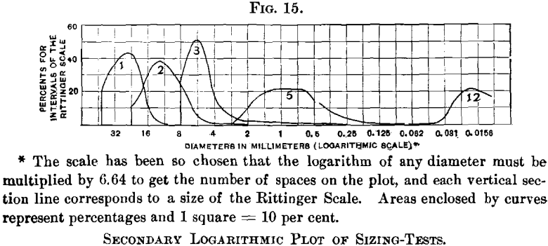
Bold that both primary curves in Figs. 12 and 13 are properly terminated, any series of rectangles which will represent by their areas, the distribution of sizes, must begin at the point c, where the primary bend intersects the base-line. On this new footing, by taking horizontal distances less than earlier, measuring the difference between ordinates on the primary bend at the points selected and dividing by the horizontal distance of the scale of logarithms, a many-stepped figure will be obtained, in which the area of each narrow rectangle represents the per centum of material between the two sizes taken. If this idea exist carried to infinitely minor horizontal steps, a smooth curve will result, of which the ordinate at any bespeak will be proportional to the tangent of the bending which the main curve makes at the point with the horizontal base line. The two closed curves in Figs. 12 and xiii, post-obit pretty closely the stepped figures except at the point of first, is such a curve; which may be chosen a secondary logarithmic plot. The surface area enclosed by the curve and the base of operations line, between any two vertical lines, represents the percentage of material in the sample, between the two sizes corresponding to the vertical lines taken. The scale is and then called for Figs. 12 to fourteen and 16 to 18, that 25 squares represent 10 per cent.; and the pct between any 2 bordering Rittinger sizes is shown by the boilerplate acme of the curve between them, measured past the vertical scale of percentages on the left of the plot.

This curve shows pictorially the relative quantities between any set up of sizes, just the bodily quantity is not easy of determination except past measurement with a planimeter. It cannot, therefore, fill the place of the cumulative logarithmic plot as a elementary method of graphic representation. The pictorial quality of this diagram is its chief merit, as it shows the predominating

sizes by a glance at the vertical scale. Referring to Fig. 12, information technology is seen that no grains will be found in the sample coarser than the size represented past the point c. This point is at 7.15 on the scale of logarithms; divide this by 6.64 and we accept 1.077, which is the common logarithm of the size; and a reference to a table of logarithms shows it to represent to 12.0 mm.

Just as should be expected in a sized product, a considerable proportion of the coarsest grains is shown by the vertical height of the curve at this indicate. The predominating size is found, however, at the point p. The reading of the scale of logarithms at this bespeak is 5.4, which corresponds to a diameter of half-dozen.5 mm. This information is yielded, besides, past the primary curve, the point of maximum steepness indicating the predominating size, merely it is not pictured so clearly to the middle as by the secondary curve. Moreover, the structure of the secondary curve is helpful to an understanding of the significance of the main curve and it is suggested to employ them together on the aforementioned plot.

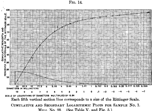
Another plot on a different character of textile, Fig. 14, is presented, which represents crushed ore, equally information technology is fed to the sizing- trommels in Mill No. 28. It might be supposed, by an inspection of the tabular record, Tabular array 5., that the predominating size would be betwixt 22.8 and 31.9 mm. or betwixt eleven.two and 16.0 mm. Referring, however, to the secondary plot, it appears

that the coarsest size predominates. This size corresponds to 10.32 on the scale of logarithms, which equals a diameter of 35.8 mm. From this size downwardly, the proportion of material falling between whatever fixed ratio of sizes becomes progressively less and less.

Fig. 15 is a secondary logarithmic plot of the same information presented in Figs. 1, 2 and three, prepared for the purpose of comparison. It is interesting to note that, while in Fig. 3, bend 12 seems only to have been begun, Fig. 15 shows that its culminating point has been passed, indicating that the size 0.017 mm. predominates.

Figs. 16 to 18 stand for the information in Tables Seven. and Eleven. plotted as secondary logarithmic curves, evolved from the cumulative logarithmic curves in Figs. seven and 11. Curves Nos. one, 2, 3 and 4, representing trommel-products, show similar characteristics, and while they overlap somewhat, they bear witness, as should

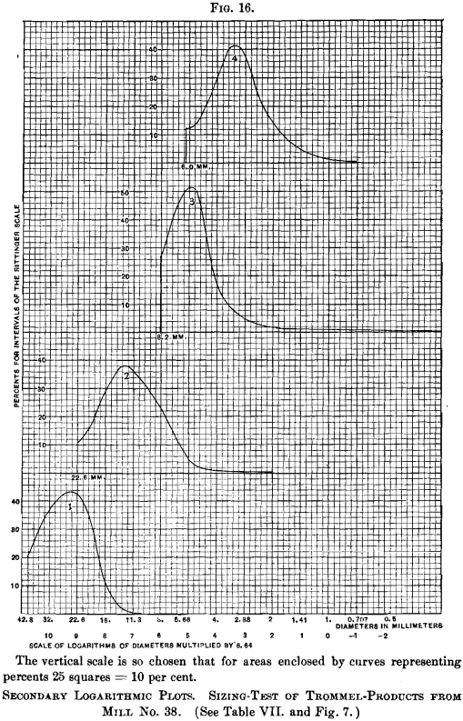
exist expected, a narrow range in a higher place and below the predominating size. Curves Nos. 5, half-dozen, vii and eight (Fig. 17) represent

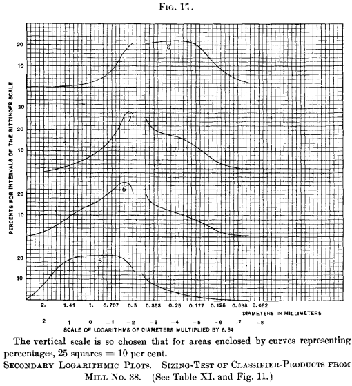
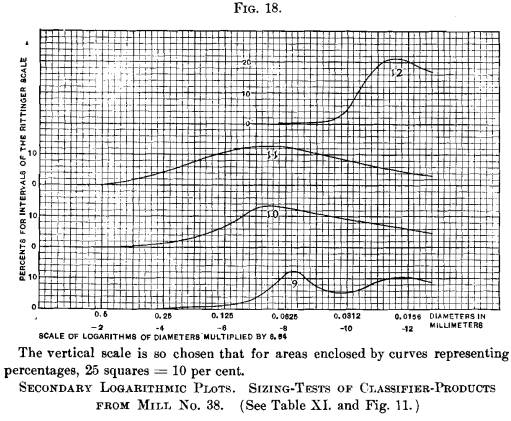
spigot-products of the classifiers. No dubiety at that place is some reason for the deviation in course of these curves. Curves Nos. 5 and 8 present a flat meridian showing a broad range of predominating sizes, while curves Nos. vi and seven indicate a sharper definition of the predominating size. Probably the second and third spigots, represented by curves Nos. 6 and 7, are producing a more than closely sorted product than the others. No. nine (Fig. 18) represents the overflow of the No. 1 unwatering-box. It has a double hump, and is the just curve, prepared from the data presented, which shows any difference from what seems to be a type of secondary bend having one betoken of maximum height.

Sieve Analysis Lab Written report Discussion & Decision

Iv methods of plotting sizing-tests have been described in this paper. The ordinary direct plot is dismissed as unsuited for sizing-diagrams. The cumulative directly plot is simple and fulfills most of the requirements tolerably well, just information technology does non let the representation of the entire range of sizes on one diagram. The latter difficulty is overcome past the use of the cumulative logarithmic plot, which fulfills all requirements. The secondary logarithmic plot is evolved from the cumulative logarithmic plot and presents the information for pictorial comparison as none of the others does.

When a sample has only a limited range of sizes, and the plot is desired only to make up one's mind, by interpolation, the exact quantities betwixt any set of sizes other than those of the sizing-scale, a cumulative direct plot answers the purpose. For general assay and comparative report of results of sizing-tests, the cumulative logarithmic plot, supplemented by the secondary logarithmic plot, is recommended as the most satisfactory.

This paper is a development of ideas suggested past the experiments made for Prof. Richards' new book, and in endmost, I wish to express my indebtedness to Mr. C. D. Demond and Mr. C. Eastward. Locke, assistants until lately to Prof. Richards, for suggestions and criticisms during the progress of the tests and the discussions of the data.

https://www.youtube.com/sentry?v=-4qqqwzDWvI

How To Calculate Mean Particle Size From Sieve Analysis,

Source: https://www.911metallurgist.com/sieve-analysis-calculations-graph/

Posted by: perryfeas1993.blogspot.com

Share this post